Detecting Anomalies using Machine Learning on Splunk

By Paulo Matana da Rocha

Introduction

Detecting cyberattacks is essential to ensuring the security of networks and systems. Therefore, in order to detect malicious activity, many companies use security information and event management (SIEM) platforms to gather, manage and analyze data from different log sources, such as firewalls and operating systems. In general, malicious activity can be discovered by implementing detection rules in SIEMs that check for patterns of activity or code corresponding to attacks, i.e. signatures of malicious activity. However, although detecting attacks using signatures works well for many situations, it also presents some problems and limitations, such as difficulty in detecting variations of attacks or unknown attacks, since there are no specific signatures for them [1].

In order to overcome these limitations, another detection approach is increasingly being adopted: anomaly detection. Anomaly detection systems model the normal behavior of users, networks and systems in order to establish normal patterns and measure deviations from these parameters, since large deviations represent non-conformities with normal behavior and therefore indicate suspicious activity [2]. In this context, the use of machine learning algorithms has shown promising results in anomaly-based cyber-attack detection. They don’t rely on known attack signatures, but on observing and identifying patterns in the data, learning the regular characteristics of system and network data in the absence of malicious activity and even the behavior that occurs during attacks [3, 4]. We invite you to read our series of blog posts Empowering Intrusion Detection Systems with Machine Learning, in which we cover how different machine learning algorithms can be used to detect cyberattacks.

But how do you implement, train and run machine learning algorithms in SIEMs? Fortunately, the main SIEM companies on the market have already realized the advantages and benefits of using machine learning to detect cyberattacks, and have provided specific tools for this purpose. In this blog post, we’ll explain, in a practical and objective way, how to implement, train and put into practice attack detection using machine learning in the Splunk SIEM through its Splunk App for Data Science and Deep Learning (DSDL) tool, formerly known as the Deep Learning Toolkit (DLTK) [5]. All the code created in this blog post is available at https://github.com/tempestsecurity/splunk_dsdl_tutorial.

Splunk DSDL

DSDL is a Splunk tool that integrates it with a container in which we can implement machine learning algorithms developed on a Jupyter Notebook with the main machine learning and deep learning libraries and frameworks, such as scikit-learn, Pytorch and Tensorflow. In this way, we can implement several existing machine learning algorithms that are widely used in anomaly detection, as well as develop and implement our own algorithms. In addition, the container can be run in a docker on a different device from the one Splunk is running on, allowing, for example, the use of systems with AWS GPUs to have greater processing capacity for training machine learning models. Image 1 illustrates the Splunk DSDL architecture. For more information, please see [6].

Installing Splunk

So, let’s start our tutorial. First of all, we need to install Splunk. Although this is a paid tool, you can use it for free for 60 days by signing up for a free trial. In fact, even after these 60 days, you can continue to use Splunk with a slightly more limited version, but one that is sufficient for the examples we are going to do in this tutorial.

So, access the official Splunk website https://www.splunk.com/, create an account and log in. Then, as shown in Image 2, click on “Products -> Free Trials & Downloads”.

Next, choose the “Enterprise” option, as shown in Image 3, and download the option that suits your operating system, as shown in Image 4.

Finally, follow the installation instructions in the Linux installation manual, if you are using Linux, or in the main installation manual if you are using other operating systems.

Starting Splunk

Once installed, start Splunk according to the steps listed below.

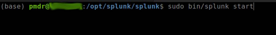
1. Open the terminal, navigate to the directory where Splunk was installed and run the command:

$ sudo bin/splunk start

2. At the end of the previous command, access the Splunk server link using a browser (ctrl+click on the link usually works).

3. Log in with the username and password registered during the Splunk installation.

Installing the DSDL

Now we need to install the DSDL and its requirements:

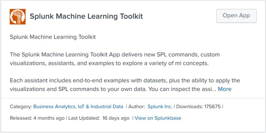
• Machine Learning Toolkit (MLTK)
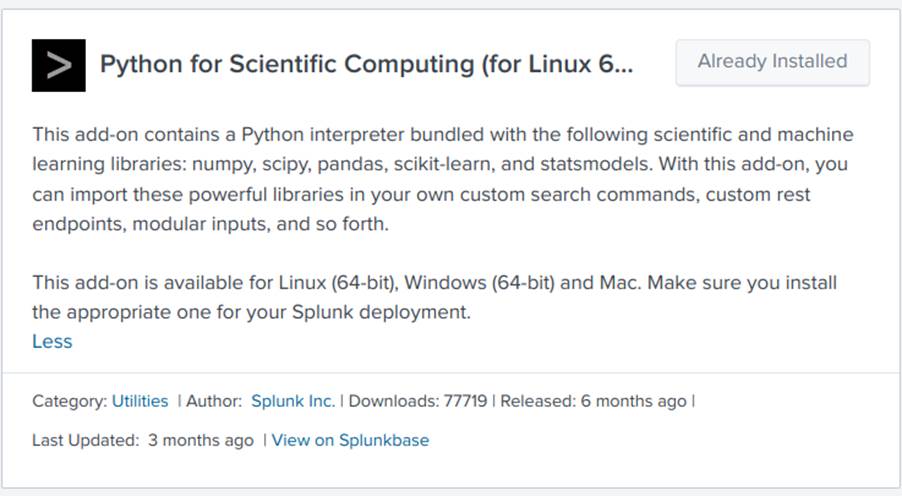
• Python for Scientific Computing

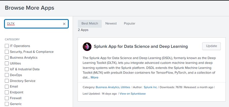
So, in Splunk, click on “+ Find More Apps” as shown in Image 8 and search for the names of the Python for Scientific Computing, MLTK and DSDL apps, as shown in Image 9, and install them as shown in Images 10, 11 and 12.

Configuring the Container

As mentioned, DSDL works in a container. So now let’s see how to configure it.

First of all, we need to install docker on the machine where the container will run, according to the instructions at https://docs.docker.com/get-docker/.

After installing docker, follow the steps below:

1. Run the command below to download the image that will be used by the container.

sudo docker pull phdrieger/mltk-container-golden-image-cpu:5.0.0

2. Add permissions to docker with the commands

a. Add a group to docker:

sudo groupadd docker

b. Set the permissions:

sudo usermod -aG docker $USER

c. Log out and then log in to the system or use the command

newgrp docker

d. Check if you can run commands without running sudo

docker run hello-world

If you have any questions or need more detailed information, go to https://docs.docker.com/engine/install/linux-postinstall/

3. Finally, start the container with the command

docker run phdrieger/mltk-container-golden-image-cpu:5.0.0

With the container running correctly, all you have to do now is finish the setup inside the DSDL. To do this, follow the steps below:

4. On the App DSDL home screen, go to “Configuration->Setup” as shown in Image 14.

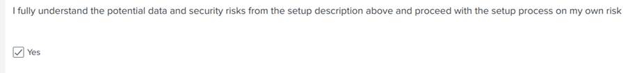
5. Check the box agreeing to the risk, as in Images 15 and 16.

6. Finally, fill in the fields in Image 17 as described below:

a. Docker Host: unix://var/run/docker.sock

b. Endpoint URL: localhost

c. External URL: hostname  (can be found by running the $hostname command in the terminal)

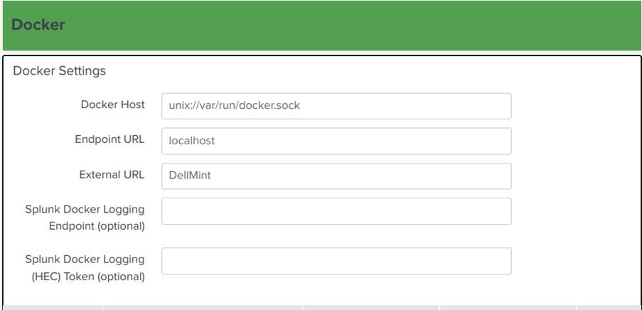
7. Click on Test & Save at the bottom of the page.

Creating Detection Models using Machine Learning

Finally, we’re ready to implement detection models using machine learning in Splunk. Now let’s see how to do it. To do this, we’ll need data and a detection algorithm.

Obtaining data

In this blog post, we implemented a machine learning model to detect anomalies in firewall logs. We used a database of firewall logs available in Splunk. So, let’s first find this database and make sure it can be accessed by the DSDL using the following steps:

1. Click on settings in the top bar of Splunk;
2. Click on Lookups, as shown in Image 18;
3. Click on Lookup table files, as shown in Image 19;
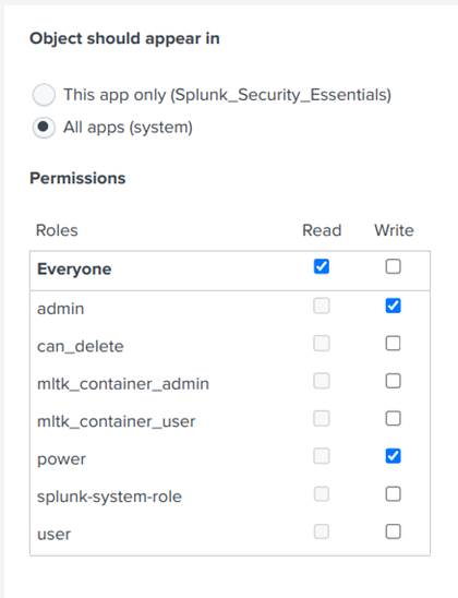
4. Search for firewall_traffic and click on Permissions, as shown in Image 20;
5. Finally, make sure that the permission settings are the same as in Image 21.

Next, we’ll learn how to search for this data, analyzing its attributes, selecting features and converting categorical variables into numerical variables:

1. Go to Splunk’s search tab, there you’ll do all the data manipulation and visualization, as indicated in Image 22. All the commands we’ll show below should be used in conjunction, to add commands to a new line just press Shift+Enter and paste the command into the line created.

   

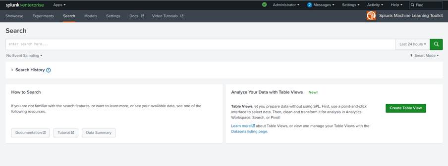
2.  For an initial view of the data, enter the query:

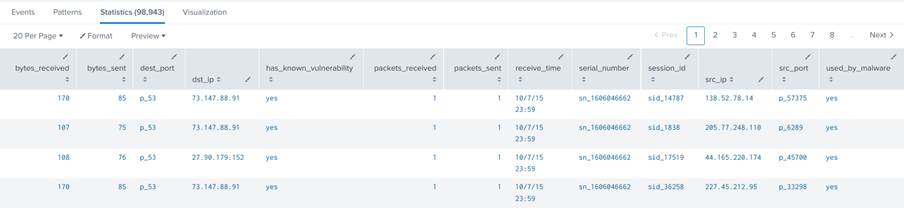
   | from inputlookup:firewall_traffic.csv

This command will return all the csv data without any processing, as illustrated in Image 23.

3. Next, to return only the fields we want, enter the query:

|fields + bytes_received, bytes_sent, packets_received, packets_sent, used_by_malware

It will return only the fields described after the “+”

4. We’ll now split the dataset into training and test sets, so enter the query:

| sample partitions=10 seed=23 | where partition_number < 7

The sample command divides the dataset into a specific number of partitions based on a seed. In this case, we create 10 partitions using the seed 23. Next, we use the where command to return only the first 7 partitions created. In this way, we split the dataset into training and test sets using the ratio 70% training and 30% test.

5. The field used_by_malware will be used by the model, but it’s categorical and needs to be converted to numerical values. To do this, use the queries:

| eval used_by_malware_yes = case(used_by_malware == "no", 0, used_by_malware == "yes", 1)
| eval used_by_malware_no = case(used_by_malware == "no", 1, used_by_malware == "yes", 0)

These commands convert the categorical field into two new numeric variables with the same information.

6. We may see some fields with no value in the dataset. To deal with them, add the command:

| fillnull value=0

This will fill in the null values with the value 0.

7. Finally, to generate a table containing only the values of the attributes we are interested in, add the command:

| table bytes_received, bytes_sent, packets_received, packets_sent, used_by_malware_yes, used_by_malware_no

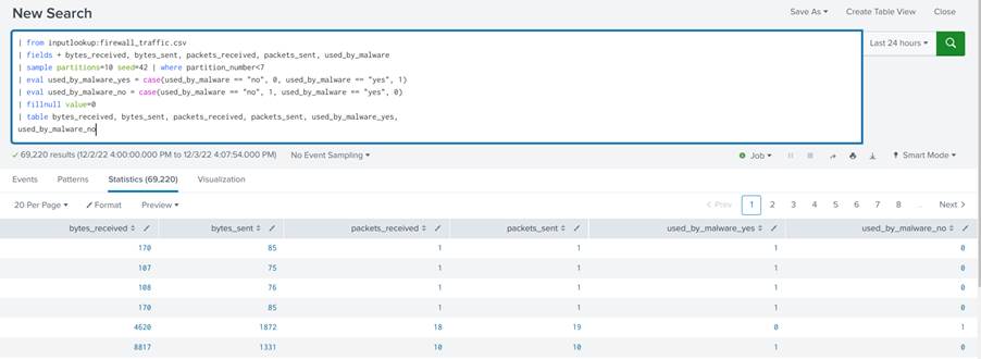
The complete query, composed by joining the queries shown above, looks like this:

| from inputlookup:firewall_traffic.csv
|fields + bytes_received, bytes_sent, packets_received, packets_sent, used_by_malware
| sample partitions=10 seed=23 | where partition_number < 7
| eval used_by_malware_yes = case(used_by_malware == "no", 0, used_by_malware == "yes", 1)
| eval used_by_malware_no = case(used_by_malware == "no", 1, used_by_malware == "yes", 0)
| fillnull value=0
| table bytes_received, bytes_sent, packets_received, packets_sent, used_by_malware_yes, used_by_malware_no

The complete query should result in a table with the pre-processed data as shown in Image 24.

Detection model

Next, we’ll use Splunk with the DSDL module to build a model of an autoencoder, a machine learning algorithm widely used to detect anomalies.

Autoencoders are a neural network structure that works by compressing the input data, generating a smaller latent representation, and then decompressing and reconstructing it. The model learns to reduce the reconstruction error between the input and output data.  When training this type of architecture with only benign data from networks or systems, it will produce small reconstruction errors when processing benign data and large reconstruction errors when processing malicious data, since these weren’t used in the training. For more information, we suggest reading the fourth post in the series mentioned above: Intrusion Detection using Autoencoders.

Implementing the Model

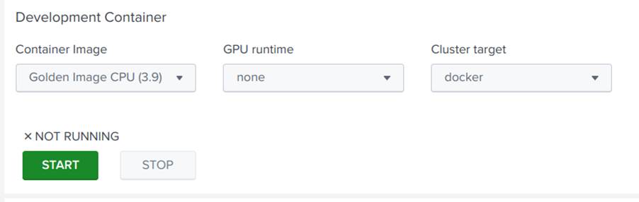
Now that we have the data, let’s implement the autoencoder model. The models used in the DSDL are made in Python using a Jupyter Notebook. To access the notebooks used in the Toolkit, go back to the DSDL home page and access the Containers option. Select the Golden Image CPU, click start, and then JUPYTER LAB, as shown in Images 25 and 26:

If you are asked for a password to log in to the notebooks, use the default password: Splunk4DeepLearning

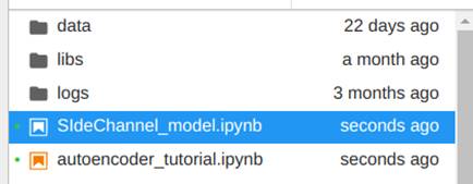
In the JupyterLab tab, open the notebooks folder and duplicate the file “autoencoder_tutorial.ipynb”. To do this, select the file, right-click on it and then click on duplicate. Now rename the copy with the name of your choice, we’ve chosen “SideChannel_model”, as shown in Images 27 and 28.

This file contains a complete tutorial on how to create a new model in DSDL. Basically, we already have an autoencoder ready. The idea now is to understand how the structure of the code works so that we can change it as we wish. But first, in order to test the code, we need the data from our search to be available to the notebook. So, to send them to the notebook, run the search made for displaying data in the previous topic and add the fit command as follows:

| from inputlookup:firewall_traffic.csv
|fields + bytes_received, bytes_sent, packets_received, packets_sent, used_by_malware
| sample partitions=10 seed=23 | where partition_number < 7
| eval used_by_malware_yes = case(used_by_malware == "no", 0, used_by_malware == "yes", 1)
| eval used_by_malware_no = case(used_by_malware == "no", 1, used_by_malware == "yes", 0)
| fillnull value=0
| table bytes_received, bytes_sent, packets_received, packets_sent, used_by_malware_yes, used_by_malware_no
| fit MLTKContainer mode=stage algo=SideChannel_model bytes_received, bytes_sent, packets_received, packets_sent, used_by_malware_yes, used_by_malware_no into app:SC_Autoencoder

This call to Splunk’s fit command indicates that Splunk should send the data obtained from the search to the SideChannel_model algorithm in the container using stage mode. The command follows with the list of data fields that will be sent to the model and the name of the model instance that will be saved, in this case SC_Autoencoder. The stage mode (mode=stage) means that the data will be sent to the development environment, where our notebook is, so we can use the data to train the model. By adding the fit command to the search, two files will be created in the JupyterLab notebook/data directory, a json file and a csv file, the former containing the configuration information sent to the model, and the latter the data.

Let’s now understand how each cell of the code in the autoencoder notebook works:

Image 29 shows the first code cell of the notebook, which contains the library imports used by the Python code and the definition of the directory where the model will be saved after it has been trained. Since only libraries installed in the container can be used, in order to use other libraries it may be necessary to build a new container with the new dependencies.

The second cell, also in Image 29, only serves to show the version of each module and is not exported to the final code.

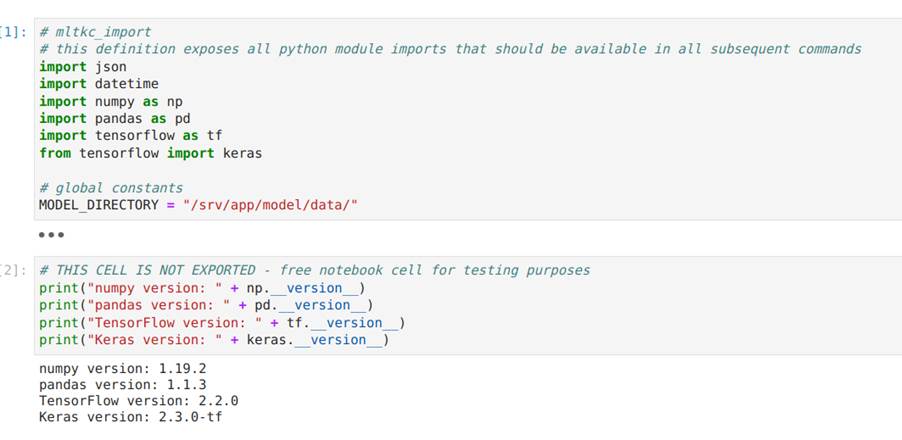
Image 29. Code cells responsible for defining packages and displaying their versions

Image 30 shows two code cells that are very important for using the notebook. The stage function is used to read the data and parameters that have been sent to the data folder. Note that the data comes in a csv format and the parameters are read as a json object. The image shows the implementation of the function and then its execution.

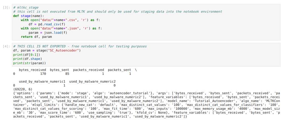
Image 30 illustrates the code cell responsible for defining the init function for initializing the autoencoder model, as well as the code cell in which the init function is called. As shown, the init function takes a dataframe with configuration parameters as input and returns the declared model as output. In this example, the model is created using the Keras library. In Image 31, we modify the init function by adding a dense layer to the autoencoder architecture just to show how simple it is to change the code.

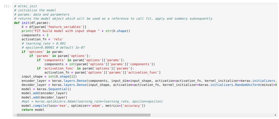
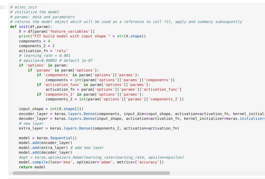
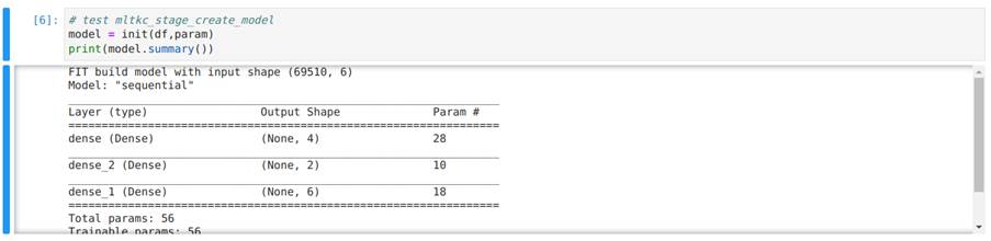
In Image 33, we execute the init function to instantiate a model and then use the summary method present in the models generated by the Keras package to show the architecture of the model created.

In Image 33, we show the implementation of the fit function which takes as input the model, a dataset and configuration parameters, and returns the trained model along with some other information. It’s important not to change the information returned to ensure that the model works correctly.

In Image 34, we train the model by calling the fit function.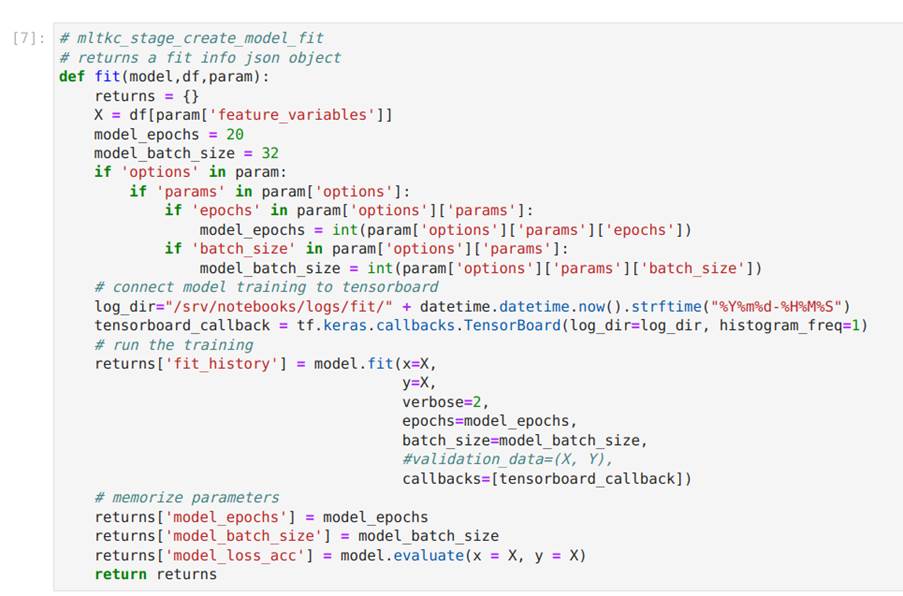

Image 34. Code cell with the definition of the fit function

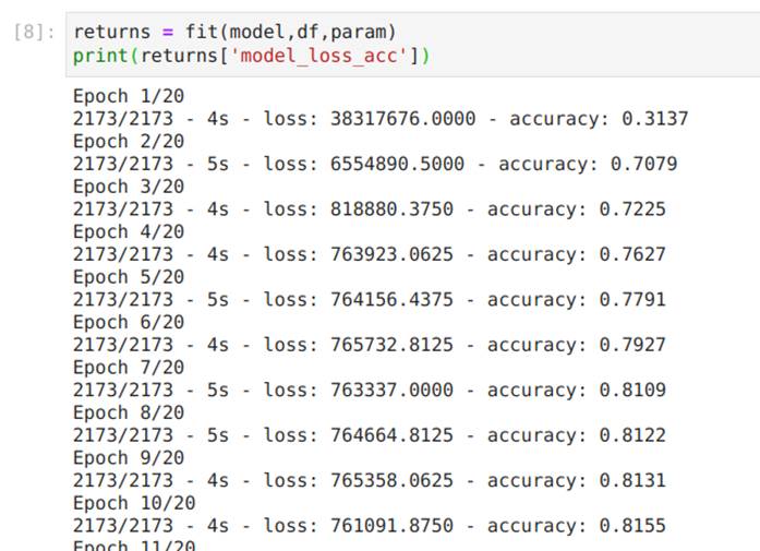
Image 36 shows the model’s apply function, which receives the model and a dataframe with parameters as input, and returns a dataframe with the model’s outputs:

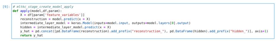
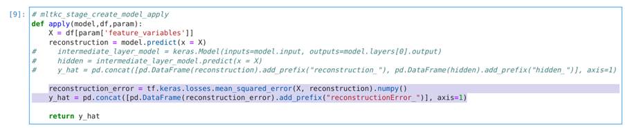
In order to detect anomalies, we changed the code in this cell by commenting out the 3 lines above the return command and adding a small piece of code that calculates the mean square error between the autoencoder’s input and output. This gives us a single value that represents the total reconstruction error of the autoencoder and is an indication of how anomalous a data sample is . The added code is described below and in Image 37:

reconstruction_error = tf.keras.losses.mean_squared_error(X, reconstruction).numpy()
y_hat = pd.concat([pd.DataFrame(reconstruction_error).add_prefix("reconstructionError_")], axis=1)

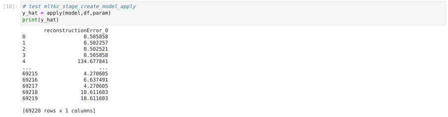
In Image 38, we test the apply function using the data:

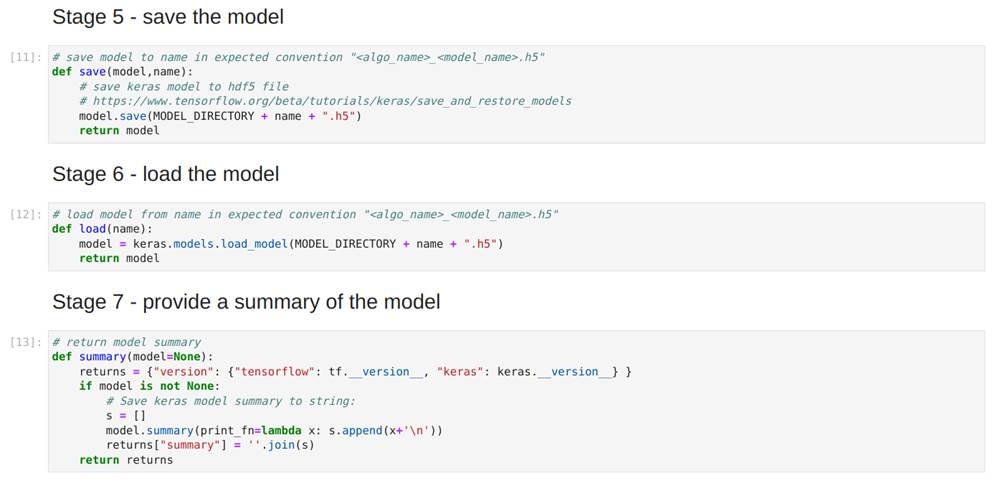
Finally, in Image 39, we see the save, load and summary functions, which save the model, load it into the environment and return a string describing the model, respectively:

The notebook containing all the changes can be found at: https://github.com/tempestsecurity/splunk_dsdl_tutorial

Using the model directly with Splunk searches:

In addition to training and applying a detection model via the Jupyter notebook, we can also train and apply it by performing searches directly in Splunk. To do this, we first need to understand how notebooks interact with searches.

We can include two commands in Splunk searches performed from the DSDL search screen: fit and apply. These commands call, in a specific order, functions from a python script that is saved in the container automatically every time the Jupyter notebook code is saved. We have 6 main functions within the template code that will be used in the python script:

• init
• fit
• apply
• save
• load
• summary

Thus, when performing a search using Splunk’s fit function (the same one used in the queries shown above), whose main objective is to train the model, a script is executed that uses the functions of the model, explained in the previous section with the Jupyter notebook, according to the diagram in Image 40.

Image 40. Splunk fit function execution diagramAfter calling the training function, to apply the trained model to the data, we use Splunk’s apply function, which in turn calls the functions explained with the Jupyter notebook according to the sequence shown in Image 41.

So, in summary, to train and apply the model using Splunk searches we just need to perform 3 steps: training with the Splunk fit function, inference with the Splunk apply function, and the definition of a detection rule:

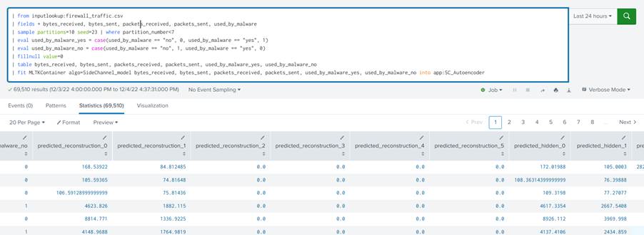
1. Training

To train the model directly using search, simply use the “fit” command in the query, but this time without passing the mode=stage argument. The “fit” command without the stage option will execute the functions in the model’s python script and save the model instance with the name given after “app:”. The sequence of functions can be seen in the diagram shown above. When training the model using search, we have:

Full query:

| from inputlookup:firewall_traffic.csv
| fields + bytes_received, bytes_sent, packets_received, packets_sent, used_by_malware
| sample partitions=10 seed=23 | where partition_number<7
| eval used_by_malware_yes = case(used_by_malware == "no", 0, used_by_malware == "yes", 1)
| eval used_by_malware_no = case(used_by_malware == "no", 1, used_by_malware == "yes", 0)
| fillnull value=0
| table bytes_received, bytes_sent, packets_received, packets_sent, used_by_malware_yes, used_by_malware_no
| fit MLTKContainer algo=SideChannel_model bytes_received, bytes_sent, packets_received, packets_sent, used_by_malware_yes, used_by_malware_no into app:SC_Autoencoder

1. Inference

Once the model has been trained, it just needs to be applied to the test data. To do this, we use Splunk’s apply command in the query and pass the name of the trained instance of the model, SC_Autoencoder, as the only argument:

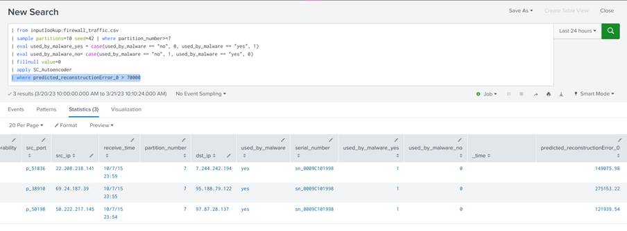
| from inputlookup:firewall_traffic.csv
| sample partitions=10 seed=42 | where partition_number>=7
| eval used_by_malware_yes = case(used_by_malware == "no", 0, used_by_malware == "yes", 1)
| eval used_by_malware_no= case(used_by_malware == "no", 1, used_by_malware == "yes", 0)
| fillnull value=0
| apply SC_Autoencoder

In the query above we load the data, take only the partitions we use for testing, do the pre-processing and finally apply the model:

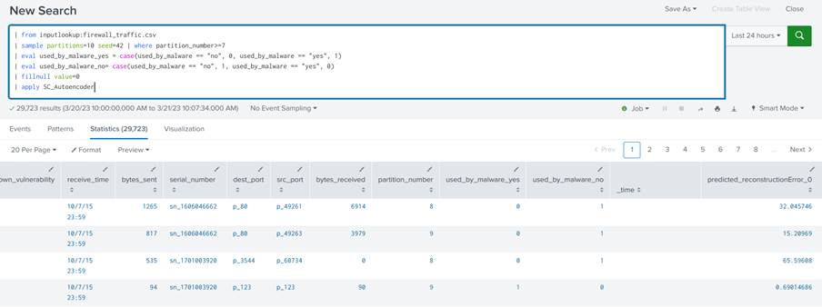
The output shows the input data concatenated with their respective predicted values.

3. Detection rule

Finally, to transform the results into a detection rule, simply add the where command to the query and specify a threshold for the field containing the reconstruction errors:

| where predicted_reconstructionError_0 > 70000

Some important tips for developing more sophisticated models:

• If your model’s apply function returns temporal data, it should be sorted in descending order;
• The models called in Splunk are executed from the JupyterLab root, so if you want to add custom modules written in Python they should be placed there;
• Since Splunk’s fit function also calls the apply, it’s ideal for conducting online training;
• You can create a customized container from the standard MLTK container repository available on github.

Conclusion

In this post, we showed you how to install and use the DSDL tool for implementing, training and using machine learning models for anomaly detection in Splunk, a topic of fundamental importance for deploying detection models based on machine learning.

References

[1] Liao, Hung-Jen, et al. “Intrusion detection system: A comprehensive review.” Journal of Network and Computer Applications 36.1 (2013): 16-24.

[2] Chandola, Varun, Arindam Banerjee, and Vipin Kumar. “Anomaly detection: A survey.” ACM computing surveys (CSUR) 41.3 (2009): 1-58.

[3] A. L. Buczak and E. Guven, “A Survey of Data Mining and Machine Learning Methods for Cyber Security Intrusion Detection,” in IEEE Communications Surveys & Tutorials, vol. 18, no. 2, pp. 1153-1176, Secondquarter 2016, doi: 10.1109/COMST.2015.2494502.

[4]Chalapathy, Raghavendra, and Sanjay Chawla. “Deep learning for anomaly detection: A survey.” arXiv preprint arXiv:1901.03407 (2019).

[5] Splunk App for Data Science and Deep Learning https://splunkbase.splunk.com/app/4607