What is Fuzzing
On a rainy night in 1988, Barton Miller, a professor at the University of Wisconsin, was accessing a Unix system via a dial-up connection, but because of the connection noise generated by the storm, he found it difficult to execute commands correctly on the terminal. What caught the professor’s attention was that the communication noise resulted in crashes in some of the operating system’s programs.
He then suggested the idea of random inputs to discover bugs in programs, a test he named fuzz, a term meaning “vague” or “imprecise”.
Following the success of the project carried out by one of the student groups, papers began to be published on this new software testing technique.
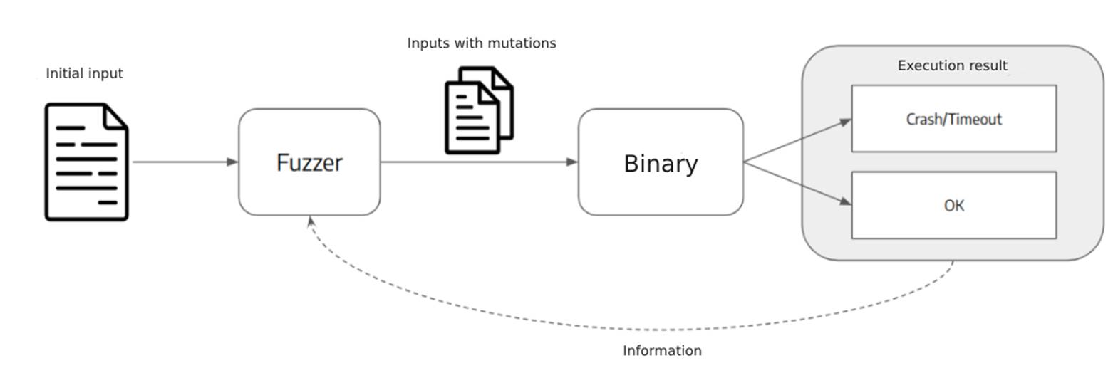
Fuzzing can be defined as a software testing technique that runs a program with several random inputs in order to cause unexpected behavior, such as crashes, exceptions or memory leaks. In general, fuzzers generate new inputs by modifying other valid ones, seeking to obtain inputs that can pass the program’s simplest validations, but which cause a problem elsewhere in the code.
A fuzzing test differs from unit tests due to the fact that unit tests use inputs already created for the test, which can be valid or invalid, observing whether the tested part of the code shows the expected behavior. Fuzzing tests, on the other hand, usually generate a large number of random inputs automatically, bringing greater automation to the process, as well as making it easier to identify corner/edge cases, as the inputs don’t need to be created manually by someone.
What does this have to do with security?
Many bugs found from fuzzing tests don’t just indicate that the program will get an incorrect result. Often these bugs can be signs of serious vulnerabilities. For example, an input that causes a program to go into an infinite loop can be used in DoS attacks (CVE-2019-13288) or, often, the crashes obtained in tests can indicate memory management problems, such as buffer overflows (CVE-2019-14438), which when exploited can lead to the target being compromised.
A quick search on the internet shows numerous CVEs discovered with the help of fuzzers. Even some vulnerabilities that have remained “hidden” for many years, such as the sudoedit vulnerability (CVE-2021-3156), could have been found using modern fuzzers such as AFL++. [6]
“Need” for Feedback
Some more advanced fuzzing tools don’t modify inputs in a totally random way, but mutate the input taking into account information (feedback) obtained from the execution of old inputs. In other words, the fuzzer (the tool that runs the test) tries to generate inputs intelligently in order to test as much of the code as possible.
There are various metrics that can be used by the tool to assess how “interesting” an input is. Some possible metrics are:
- number of lines of code executed;
- number of machine code (assembly) instructions executed;
- number of functions executed;
- number of memory operations performed (malloc, calloc, free, memcpy, …).
The idea is that the fuzzer uses one of these metrics as feedback on the execution of a specific input and, by comparing the result of several inputs, can identify those that cause a difference in the target’s behavior and use them as the basis for new mutations. And new inputs that cause no change in the metric can be discarded.
We can illustrate the idea of feedback by taking the example of fuzzing in the pseudocode below:
vetor = read_input(); //reads 4 integers as input

if(vetor[0] == 0x24)
	if(vetor[1] == 0x3F)
		if(vetor[2] == 0x6A)
			if(vetor[3] == 0x88)
				vulnerable_code();
The code reads four integers as input (32 bits each), performs some nested comparisons and, if the input passes all the tests, the function ” vulnerable_code” is called, which illustrates a possible vulnerability.
A fuzzer can generate entries randomly, in the hope that at some point it will generate an entry that finds the vulnerable code. In the example above, the probability of each fuzzer entry finding the vulnerable code is very low, around 1 in ~4 billion, because the chance of randomly hitting each byte is 1 in 256, and as there are four bytes, the chance of hitting all four at the same time is 1 in 2564.
The tool becomes more efficient if you consider which lines were executed for each input. For example, for an input of (0x00, 0x00, 0x00, 0x00), the program above will only execute the first “if” and will finish execution, while for an input of (0x24, 0x00, 0x00, 0x00) the program will also execute the second “if”. By analyzing this behavior, i.e. the code coverage reached by each input, it’s possible to explore other areas of the code more quickly.
In this example, the fuzzer can see that by changing the first input to “0x24” a new part of the code is executed, so it can keep the first input fixed at “0x24” and start changing the second input until a different behavior occurs, and so on.
With this, our fuzzer wouldn’t need to test all ~4 billion combinations to find the vulnerability, but only 1024 combinations, as it would end up considering each input separately.
How does AFL++ work?
There are several fuzzers, but this article will focus on AFL++ (American Fuzzy Lop plus), explaining both how it works theoretically and demonstrating, through an example, how it can be used to search for vulnerabilities in open-source programs.
AFL++ is a mutative fuzzer based on feedback, which means that it modifies the generated inputs not in a totally random way, but in an attempt to find new pieces of the program that are still unexplored.
Branch Coverage
The metric used by AFL++ as feedback on the execution of an input is branch coverage [4]. The image below is a simplified illustration of a program in which each block is a linear sequence of instructions and whenever a jump occurs, the program executes another block of code, which is represented by an arrow connecting the two blocks. The arrows can be blue, in case the program always executes the same block of code, or red and green, when the flow of the program can vary, as in a comparison instruction that executes different parts of the code depending on the result obtained.
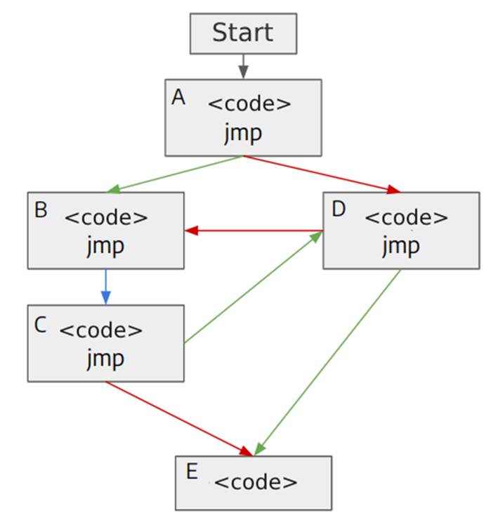
Two possible execution sequences for this program are:
1 – A, D, B, C, E
2 – A, B, C, D, E
In both cases, the same number of code blocks are executed, i.e. the two sequences go through the same instructions, call the same number of functions, perform the same memory operations, etc. Therefore, all the metrics discussed in the previous section would obtain the same result for the two executions, since the only difference is the order in which the code blocks are executed.
However, a change in the order of execution can cause problems if the developer has not anticipated this possibility and, in order to be able to distinguish cases like this, AFL++ does not consider which blocks of code were executed, but rather an idea of a “tuple”.
A tuple is nothing more than a link between two blocks of code. The tuples in the two execution sequences above are:
1 – A-D, D-B, B-C, C-E
2 – A-B, B-C, C-D, D-E
With this, the fuzzer can differentiate between the two execution sequences, because it’s interested in which “path” or “branch” the program took. Hence the name “branch coverage”.
In addition, AFL++ counts the number of times each tuple has been executed, and stores this count in “buckets” [1, 2, 3, 4-7, 8-15, 16-31, 32-127, 128+]. The advantage of not considering the exact number of executions, but rather the buckets, is that this action avoids path explosion, because for a tuple that has always been executed only once and is now executed twice, there’s a significant difference. However, for a tuple that was executed 98 times and is now executed 99 times, it’s unlikely to present a significant change in the flow of the program, and this difference can be ignored.
In short, AFL++ considers an entry to be “interesting” if it finds a tuple that has never been executed by the fuzzer before, or if the count of a known tuple has changed enough to change bucket.
Instrumentation
It’s through instrumentation of the target binary that AFL++ obtains branch coverage. There are different techniques that can be used depending on a number of factors, such as the binary’s platform (Linux or Windows), whether we have access to the source code, etc. In this article, the focus will only be on the case where we have the code and can compile the target with one of the AFL++ compilers.
The instrumentation that is inserted into the target program is responsible for obtaining the branch coverage and keeping count of how many times each tuple has been executed. The code inserted into each branch can be approximated by the snippet below. [5]
 cur_location = <COMPILE_TIME_RANDOM>;
 shared_mem[cur_location ^ prev_location]++;
 prev_location = cur_location >> 1;
Source: https://lcamtuf.coredump.cx/afl/technical_details.txt
The identifier for each location is generated randomly using compile time. The shared_mem vector is a memory region passed to the target binary, each byte of which can be considered to represent a specific tuple.
Simply put, the instrumentation identifies each branch with a random ID and, whenever execution reaches one of these points, it increments a value in the bytemap at the address resulting from the XOR operation of the ID of the current point in the code with that of the previous one, the address representing that tuple.
The last line performs a bit shift on the ID of the current location, this trick allows the instrumentation to differentiate between tuples A-A and B-B, since the XOR operation between two equal values always results in zero. [5]
Harness, Code Patches and Persistent Mode
When you have access to the source code, using the AFL++ compilers solves the instrumentation problem, but sometimes the fuzzing target can’t be tested directly. This is the case, for example, when fuzzing a library that receives no input, but must be imported and used by other programs, or when you only want to test a specific part of a large program. In both cases, you need to create a binary to be the target of the fuzzing; this binary is called a harness.
The harness, then, is nothing more than a program which will receive the inputs from AFL++ and perform the necessary preparations and treatments so that the fuzzing target is tested correctly.
AFL++ also has an execution mode called persistent mode. In this mode, which requires changes to the source code, the fuzzer doesn’t need to restart the entire execution of the program to test each new test case, instead it uses a snapshot to take advantage of the initialization of the target already executed in previous entries. For example, we could target a program that parses an image. As soon as it runs, it spends some time initializing, then it reads the input file and performs the parsing and, finally, it performs a “cleanup” before closing the program, which also takes time. So, what you can do is run a loop during this intermediate period of execution – which involves reading the input file and parsing it – so that you can test several different inputs with just a single initialization.
Other changes to the code can also speed up the fuzzing process on the chosen target. It might be interesting to study how the program works in order to identify cases where a patch in the code could be helpful.
Initial corpus and mutations
To start the fuzzing process, AFL++ needs a set of valid entries for the target binary or harness. This first set of entries is called the initial corpus and, ideally, it should contain entries that are small but exploit as many of the target’s features as possible. The fuzzer creates new entries by mutating the corpus. AFL++ has three mutation stages, “Deterministic”, “Havoc” and “Splice”. Let’s take a look at them.
The first stage is called Deterministic because it’s decisive, and in it the fuzzer performs a specific sequence of mutations, which involves, for example, inverting all the bits of the input, and inserting “interesting values”, which are values that are related to some common problems to be encountered, such as overflows.
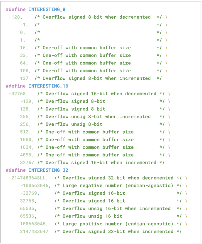
Source: https://github.com/AFLplusplus/AFLplusplus.
The second stage is called “Havoc“, a word that means “widespread destruction” or “devastation”. In this stage the fuzzer inserts, modifies or removes totally random byte sequences in parts of the input.
In the third stage, called “Splice“, the fuzzer combines two different inputs into a new one.
Overview
The image below illustrates a simplified overview of how AFL++ works.
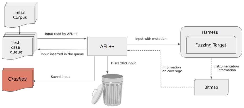
Simplified step-by-step algorithm:
- first, AFL++ loads the test cases from the initial corpus into the test case queue;
- then it loads the next entry in the test case queue;
- mutates the input and executes the target with the mutated input;
- observes the execution feedback;
- if the mutated input found no new path in the program, it’s discarded. If a new path was found, it’s inserted into the test case queue. And if it caused the program to crash, then it’s saved for future analysis;
- returns to step 2.
AFL++ periodically analyzes the test case queue to remove obsolete entries that can be replaced by new ones containing greater coverage, as well as carrying out other steps with the aim of optimizing the fuzzing process [8].
Overcoming obstacles
Some programs, even with the aid of feedback, have parts that are particularly difficult to reach with random inputs. Among these obstacles are comparisons with very large integers (32 or 64 bits), string checking, checksums, magic byte validation, and many others. As an example, the code snippet below compares the user’s input with a 32-bit integer. In order for the fuzzer to execute the unsafe code within the if, it needs to get all 32 bits right at once, because whether the fuzzer generates incorrect inputs close to the correct value such as “0xabad1deb” or bad inputs such as “0x00000000”, the branch coverage(feedback) is always the same.
if (input == 0xabad1dea)
/* unsafe code */
else
/* safe code */
Due to obstacles like these, several techniques have been developed in order to assist the fuzzing process.
Dictionary
AThe first technique is the use of dictionaries. A dictionary in the context of fuzzing is a set of tokens that have some special meaning for the program being tested. The fuzzer then uses these tokens during input mutation, increasing the chance of generating an input that changes the application’s behavior.
The image below illustrates some of the symbols in a JSON dictionary.
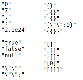
In addition, you can create a list of all the strings in the program – by running the strings utility on Linux, for example – and use this list as a dictionary, increasing the chance that the fuzzer will be able to pass comparisons with hard-coded values.
Laf-Intel
Another technique is known as “Laf-Intel”. The focus of this technique is to break down difficult comparisons so that the fuzzer can pass in smaller ones. Below are two code snippets that in practice do the same thing, i.e. execute the unsafe code when the input value is equal to “0xabad1dea”. However, the first code does this in a single comparison, while the second performs four nested comparisons. [13]
if (input == 0xabad1dea)
    /* unsafe code */
else
    /* safe code */

if (input >> 24 == 0xab)
    if ((input & 0xff0000) >> 16 == 0xad)
        if ((input & 0xff00) >> 8 == 0x1d)
            if ((input & 0xff) == 0xea){
                /* unsafe code */
                goto end;
            }
/* safe code */
end:
The advantage of the second code is that if the input generated by the fuzzer has the correct first byte (0xab), the code goes on to perform the second comparison and, if the second byte (0xad) is also correct, it will perform the third comparison, and so on, generating a different branch coverage for each byte that the fuzzer “got right”. In this way, the fuzzer once again utilizes the benefits of feedback.
Code Patching
Some codes perform checksums and other types of complex checks or validations on the input, so AFL++ would have a hard time generating a valid input. In these cases, a possible way out is simply to remove these checks from the source code and compile the target binary without these checks. Just remember to test any crashes found in a binary compiled with the checks (you may need to make some manual modifications to the input) to see if the vulnerability really exists, or if it arose because of changes to the code.
RedQueen (Input-to-State Correspondence)
RedQueen is the implementation of a technique that takes advantage of the fact that comparisons and checksums are often carried out using pieces of input. In other words, the values that are in memory or registers, at a given point in the execution, are taken from the input without any transformations or just by undergoing some simple transformation. The authors of the paper call this correlation “Input-to-State Correspondence”. [9]
To illustrate the idea behind this technique in a simplified way, let’s consider a program that checks the Magic Bytes of the input file. This particular program reads the first few bytes of the input and compares them with “ABCD”.
Let’s assume that the fuzzer initially sends an input containing the bytes “0xAABBCCDDEEFF” and monitors the state of the program when it encounters comparison operations:
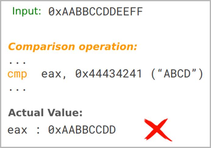
In the example above, the program compares the contents of the “eax” register with “0x44434241”, but the value contained in the register in this execution is “0xAABBCCDD”. The fuzzer creates a substitution rule and swaps “0xAABBCCDD” for “0x44434241” in the input, hoping that this value from the register was read directly from the input.
If the substitution is successful, a future run will successfully pass the check, as shown below:
Sanitizers
Programs written in C/C++ often have problems with memory management that can lead to security risks. However, these errors often don’t cause a crash, so AFL++ can’t detect when one of these issues is present.
To solve this limitation, tools known as “sanitizers” can be used, such as ASan (AddressSanitizer).
ASan detects some memory errors, such as buffer overflows, use after free, memory leaks etc, at runtime, even when these errors don’t cause the program to crash. It’s a very useful tool for developers to identify memory management problems, but it can also be useful for fuzzing, as it can ‘force’ a crash whenever it finds a problem, and AFL++ will then detect it.
ASan works by replacing the memory allocation and release functions (malloc and free) with its own functions that keep track of which memory regions have been allocated by the program and which have been released. It then adds checks before every memory access or write, something like that illustrated by the pseudocode below: [7]
// ASan check
if (IsPoisoned(address)) {
  ReportError(address, kAccessSize, kIsWrite);
}

// write or read
*address = var;
var = *address;
The control of allocated and freed memory regions is done by the so-called “shadow memory”. Every 8 bytes of memory are mapped into 1 byte in the shadow memory.
When executing malloc from the ASan library, the shadow memory region corresponding to the allocated region has its values cleared, or according to the nomenclature used by ASan, the region is unpoisoned. In addition, it marks the regions around the allocated region as poisoned, which are called red-zones.
When running free, the entire shadow memory region corresponding to the freed region is marked as poisoned. And the region is added to a quarantine, so that it remains unallocated for a while.
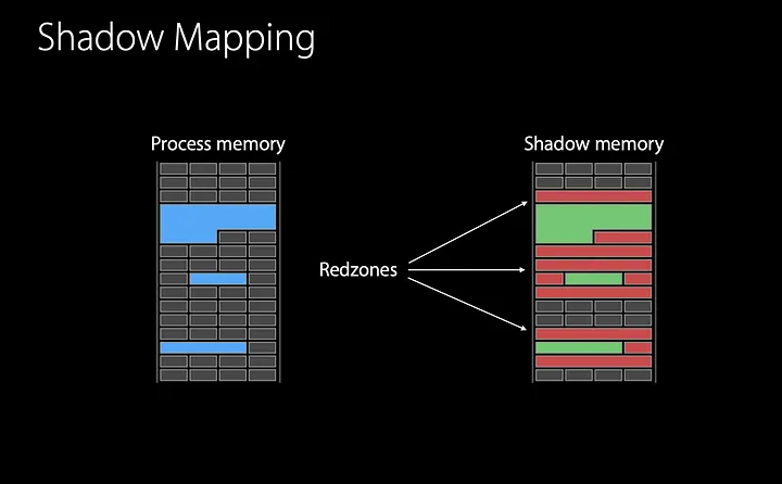
Thus, whenever the program accesses a memory region, ASan will look at the corresponding region in the shadow memory; if it’s poisoned, ASan will report an error, otherwise it will continue executing normally. This action ensures that the program only performs operations within the allocated memory region.
There are other sanitizers besides ASan, and it’s worth researching which sanitizer can help you find problems in the target you’re testing.
In Practice
To show a practical example of using AFL++, let’s try to find security problems in MPV, an open source video player. As MPV is a complex program, the focus in this practice will be on the modules that involve processing mkv files.
Instrumentation and Code Modifications
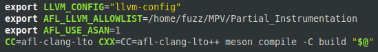
Since we had access to the source code, we used AFL++ instrumentation to obtain feedback on each run. More specifically, we used afl-clang-lto, which has some optimizations to avoid collisions when generating the random IDs that represent each block of code.
To compile and instrument the target with afl-clang-lto, some changes were made to the compilation files provided on the project’s github. The image below illustrates the changes to a section of the script, changing the compiler used and adding some flags to configure AFL++ resources, such as partial instrumentation and ASan.
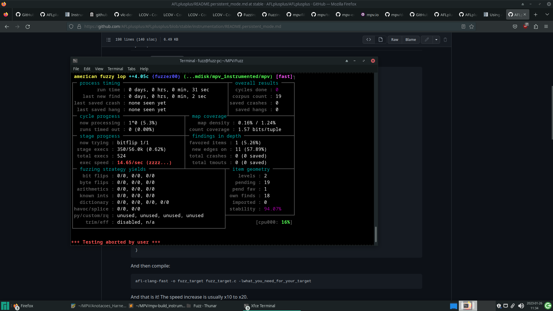
When running the fuzzer for the first time on the compiled binary, the number of executions per second was very low.
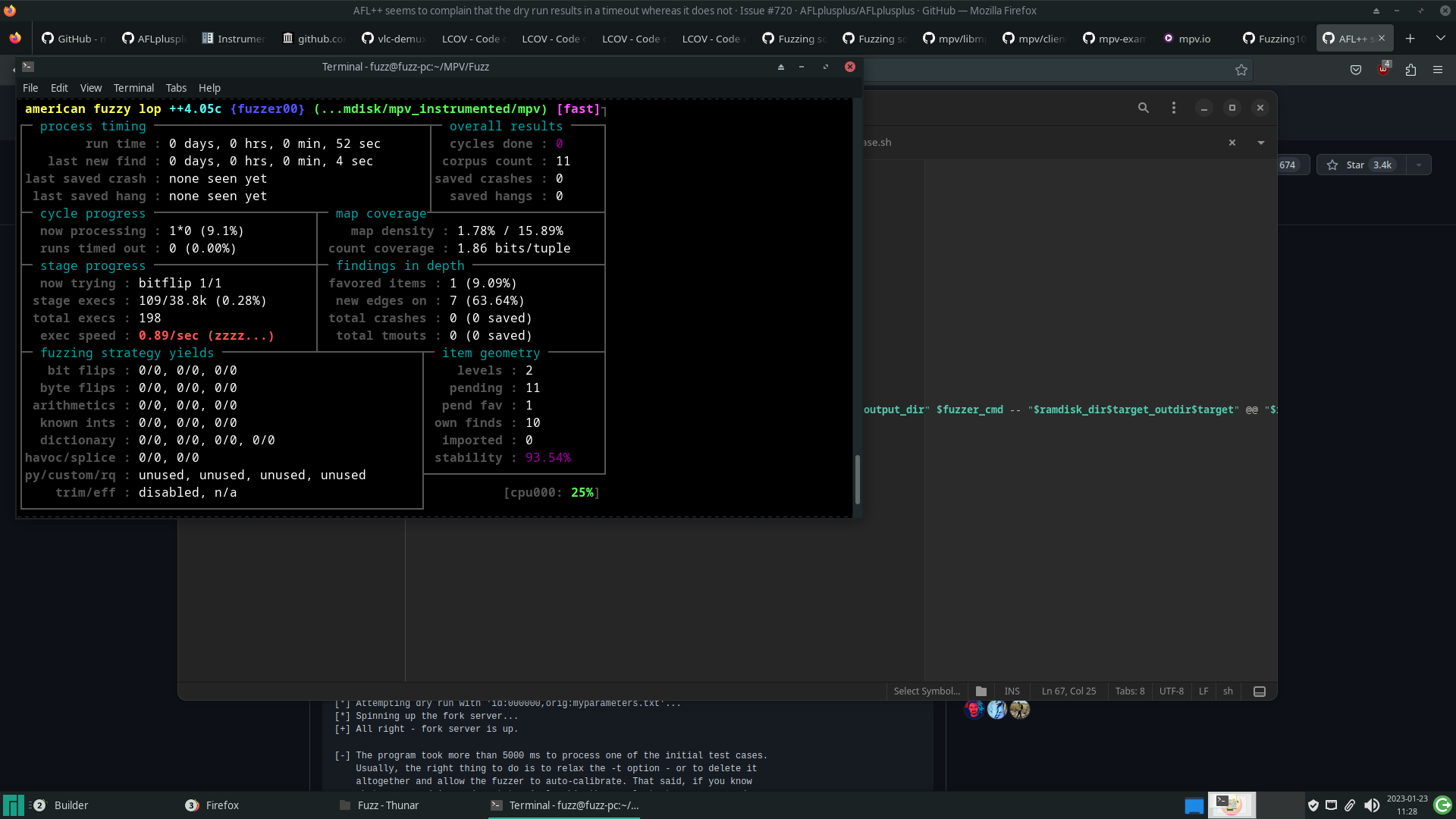
This limitation was due to the fact that, for each run of AFL++, the player performs all of its initialization, plays the video completely and finally finishes it. Carrying out this entire process for each run takes a lot of time.
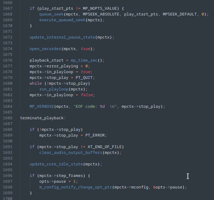
A first attempt was to change the MPV code so that execution was interrupted immediately after initialization and the first processing was carried out in the input file, illustrated by the figure below, with the addition of line 1679.
By running the fuzzer again with the above modifications, we can see an improvement in speed.
However, the program still performs the entire initialization and finalization process for each new input being executed. An alternative is to use AFL++’s persistent mode, to which a special repeat loop is added to the code, which executes the same part of the code for several different inputs, taking advantage of a single program initialization process.
The change to the code can be seen in the image below.
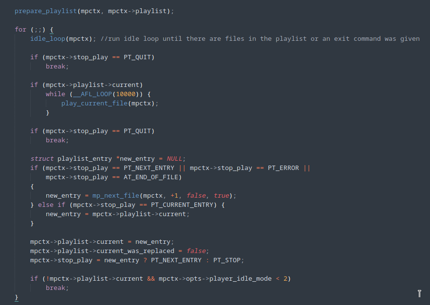
By using persistent mode, the fuzzing speed increased considerably.
Partial Instrumentation
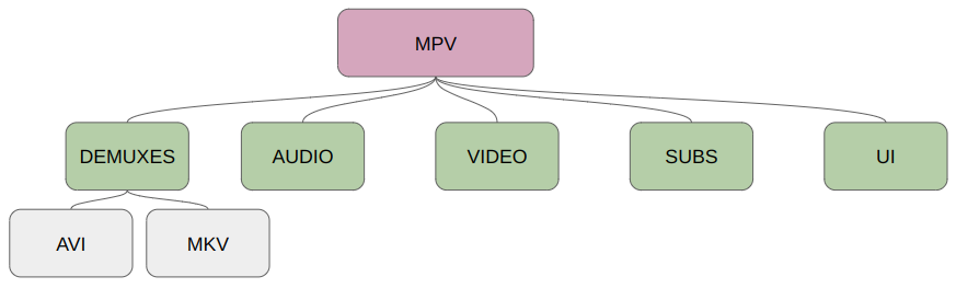
Complex programs like MPV have several files or modules responsible for different functions. Some are responsible for controlling the graphic interface, others for managing subtitles, as well as different files for dealing with the different media formats supported by the program. Because of this complexity, the fuzzer encounters a very large number of possible branches, which can greatly reduce its effectiveness.
As an example of this, we can imagine a fuzzing campaign using some MKV files in the corpus. At some point, a mutation could alter the input files so that they are recognized as AVI files. As a result, several functions specific to AVI processing are executed. The inputs are marked as interesting and added back to the test case queue. The fuzzer starts to use these “AVI” files as the basis for new mutations, so it stops focusing on the modules that process MKV, and what’s worse, it processes them very inefficiently, because these new files, despite being recognized as AVI, mostly have an MKV structure [14].
One way of keeping the fuzzer focused on specific files or functions is to use partial instrumentation. In this technique, a list of files or functions is passed to the compiler, and only these code snippets will be monitored by the fuzzer, any mutation that causes new branches outside these snippets is ignored.
As the initial focus of this fuzzing campaign is on processing MKV files, the excerpt below shows part of the list of files and functions that were monitored by AFL++ during the fuzzing process.
demux/cue.c
demux/demux.c
demux/demux_mkv.c
demux/timeline.c
stream/*.c
audio/*.c

#cue.c
fun: lstrip_whitespace
fun: read_cmd
fun: eat_char
fun: read_quoted
fun: read_int
fun: read_time
fun: skip_utf8_bom
fun: mp_probe_cue
fun: mp_parse_cue
fun: mp_check_embedded_cue

#demux.c
fun: get_foward_buffered_bytes
fun: check_queue_consistency
fun: set_current_range
Preparing the Campaign
After the changes to the code, five binaries were compiled with afl-clang-lto, using different compilation configurations:
- a binary compiled normally;
- a binary compiled with ASan;
- a binary compiled with the LFINTEL module;
- a binary compiled with the RedQueen module;
- A binary with LCOV, used to more easily monitor the code coverage obtained by the test cases.
Video samples in MKV format were also obtained to make up the initial corpus. It is interesting that these samples contain enough information for the player to execute as many code snippets as possible, but in general, the larger these files are, the slower the fuzzing process will be. Putting together a good corpus involves finding the maximum code coverage with the minimum execution overhead.
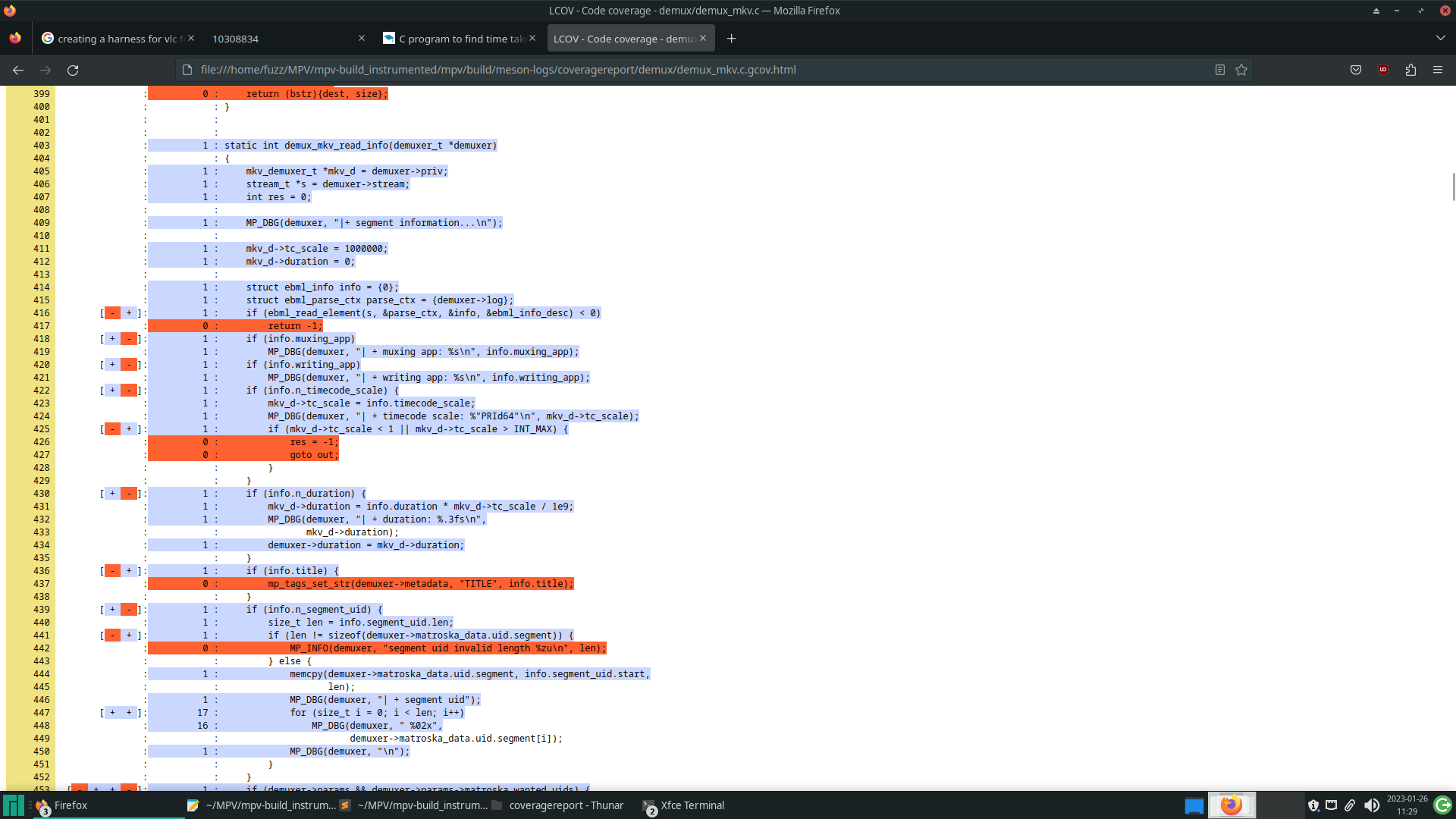
Before starting the fuzzing campaign, it’s important to validate that, after the changes, the pieces of code you want to test are still being executed, as well as evaluating the code coverage of the initial corpus. The tool used in this practice was LCOV, which is a graphical interface that obtains the results of gcov, a tool for obtaining information about the code coverage of programs, presenting them in a more readable way.
The image below shows the results of LCOV on a piece of code, obtained after executing the corpus. The lines marked in blue were executed by the program and, at the beginning of each line, there is a count of how many times it was executed
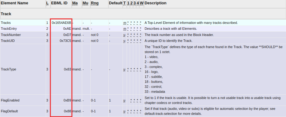
Finally, a dictionary was created containing the byte sequences that have special meaning in an MKV file.
Running the fuzzer
During campaign execution, AFL++ can perform billions of write and read operations on disk. In some cases, this can lead to premature wear on the hard drive or SSD. To get around this possible problem, we used a ramdisk, volatile storage that uses RAM to store the files and, as a result, read and write operations are performed in RAM and not on the SSD.
A script based on auto-afl [12] was used to handle the initialization of all AFL++ instances. The script helped by creating the ramdisk, initializing all the fuzzer instances, making periodic backups – remember that the process was in RAM, which is volatile memory – and optimizing the test case queue after long periods of campaigning.
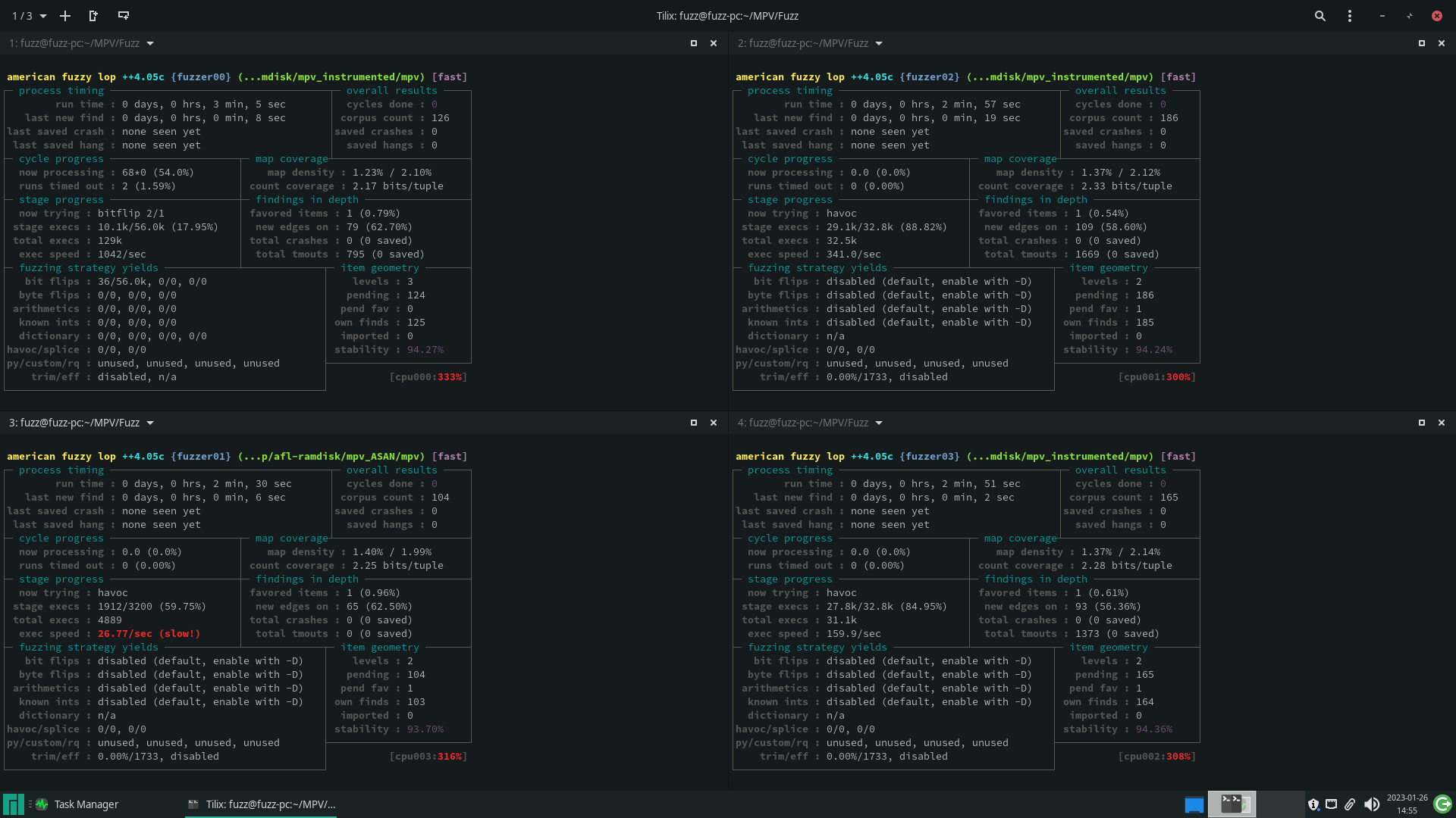
Monitoring the campaign
The AFL++ campaign provides various pieces of information about the fuzzing progress, such as the total execution time, the time since the last new discovery, the number of crashes and timeouts encountered, among others. By analyzing this information, it’s possible to assess whether the process is progressing as expected or if it’s stagnating.
If progress is not as expected, one possibility is to use tools such as LCOV again to observe the code coverage that is being achieved with the cases currently in the test queues. With this, it may be possible to identify stretches of code that the fuzzer can’t reach and manually create new inputs that make the program execute these stretches.
One way to ‘teach’ the fuzzer about these new inputs is to start a new temporary instance of AFL++ containing these new files created manually as corpus and leave it running for a while. This new instance will execute these passages that have not yet been explored by the others and, after a period of time, the other instances will synchronize with each other, obtaining the inputs based on these new inputs. After that, the temporary instance can be stopped.
Result
This fuzzing research was part of my internship at Tempest and, because of this, the campaign’s execution time was limited. After a few days of execution, no instance of AFL++ had encountered any valid crashes and different factors may have generated this result.
The first factor may have been the changes made to the source code, which were very simple. The binary as tested by AFL++ performed only some of the functions that the player would perform when playing video files and, although LCOV shows reasonable code coverage in the main files targeted by the fuzzing, a more detailed analysis of the player’s operation may result in better modifications to the code or even the creation of a harness that makes the fuzzing process more effective.
Another factor could be the length of the campaign, perhaps with a longer fuzzing time some input that executes a vulnerable piece of code could have been generated. In addition to various other details that could be improved, such as putting together a better initial corpus
References
[1] MORALES, A. Fuzzing-101. Available at: <https://github.com/antonio-morales/Fuzzing101>. Accessed on: Dec 15. 2023.
[2] Fuzzing in Depth. Available at: <https://aflplus.plus/docs/fuzzing_in_depth>. Accessed on: 15 Dec. 2023.
[3] Fuzz Testing of Application Reliability. Available at: <http://www.cs.wisc.edu/~bart/fuzz/>. Accessed on: 15 Dec. 2023.
[4] FIORALDI, A. et al. AFL ++ : Combining Incremental Steps of Fuzzing Research. [s.l: s.n.]. Available at: <https://www.usenix.org/system/files/woot20-paper-fioraldi.pdf>. Accessed on: 15 Dec. 2023.
[5] Technical “whitepaper” for afl-fuzz. Available at: <https://lcamtuf.coredump.cx/afl/technical_details.txt>.
[6] How Fuzzing with AFL works! | Ep. 02. Available at: <https://youtu.be/COHUWuLTbdk>. Accessed on: 15 Dec. 2023.
[7] Address Sanitizer Algorithm. Available at: <https://github.com/google/sanitizers/wiki/AddressSanitizerAlgorithm#short-version>. Accessed on: 15 Dec. 2023.
[8] Afl Fuzz Approach. Available at: <https://aflplus.plus/docs/afl-fuzz_approach/>. Accessed on: 15 Dec. 2023.
[9] REDQUEEN: Fuzzing with Input-to-State Correspondence – NDSS Symposium. Available at: <https://www.ndss-symposium.org/ndss-paper/redqueen-fuzzing-with-input-to-state-correspondence/>.
[10] How to Build a Fuzzing Corpus. Available at: <https://blog.isosceles.com/how-to-build-a-corpus-for-fuzzing/>. Accessed on: 15 Dec. 2023.
[11] Matroska Element Specification. Available at: <https://www.matroska.org/technical/elements.html>. Accessed on: 15 Dec. 2023.
[12] RENWAL. auto-afl. Available at: <https://github.com/RenWal/auto-afl/>. Accessed on: 15 Dec. 2023.
[13] laf-intel. Available at: <https://lafintel.wordpress.com/>.
[14] ANTONIO-MORALES. Fuzzing software: common challenges and potential solutions (Part 1). Available at: <https://securitylab.github.com/research/fuzzing-challenges-solutions-1/>. Accessed on: 15 Dec. 2023.